Measurement Uncertainty in Force Measurement

This guide outlines standardized methods for evaluating measurement uncertainty in force applications and applies these principles to load cell specification sheets. It synthesizes global practices from leading metrology journals and standard-setting bodies, including the European Association of National Metrology Institutes (EURAMET), the National Institute of Standards and Technology (NIST), ASTM International, and the Joint Committee on Guides in Metrology (JCGM).

While foundational to modern calibration, the formal concept of measurement uncertainty is relatively recent in metrology. Prior to 1977, no international consensus existed for expressing measurement uncertainty [1]. To resolve this ambiguity, the International Committee on Weights and Measures (CIPM) directed the International Bureau of Weights and Measures (BIPM) to collaborate with national laboratories worldwide. Their combined efforts produced the standardized guidelines used today across a vast spectrum of force and mass measurements [1].

The Distinction Between Error and Uncertainty

Often, the terms “error” and “uncertainty” are used interchangeably. However, their distinction is important for quantifying measurement accuracy.

Measurement error is the exact difference between an observed measurement value and the true physical value of the quantity being measured. Crucially, error is a purely theoretical concept that operators can never truly know because it is physically impossible to determine the perfect “true value” of any physical quantity. Improper load cell mounting, mechanical misalignment, or drifting calibration parameters commonly introduce systematic errors into a measurement. While operators can significantly mitigate or correct these errors through rigorous calibration, they can never fully eliminate them.

Measurement uncertainty, on the other hand, does not represent a single value. Instead, it defines a statistically calculated range of values within which the true measurement value is likely to lie, bound by a probabilistic confidence interval. In the weighing world, uncertainty represents a scale manufacturer’s confidence in how close the displayed measurement is to the actual weight on the platform. The next section will illustrate this point further.

Interestingly, the baseline uncertainty models developed by NIST explicitly incorporate physical error variables (sensor creep, hysteresis, and load alignment angle) as a single component of their combined uncertainty. Because clean laboratory procedures can suppress these individual error components, the final combined uncertainty figure in [5] is given as a “best-case” and “worst-case” range. This range directly reflects whether a laboratory operator has actively mitigated those real-world field errors through precise calibration and meticulous execution.

top

How to Interpret Measurement Uncertainty In a Load Cell Data Sheet

As a practical matter, not every application requires the highest possible accuracy, which directly correlates to higher equipment cost. The ultimate engineering goal is to source the most cost-effective tool that still meets the implementation’s accuracy requirements. To achieve this balance, a scale’s or load cell’s datasheet is the authoritative source. Here, we will look at a strain gauge load cell’s uncertainty specification, how it is derived, and what it specifically tells you about the device’s performance.

Statistically Derived Uncertainty and Confidence Intervals

A data sheet specifies a load cell’s output uncertainty as a percentage range of full-scale output (FSO). For example, consider a load cell with an FSO of \(2.2\text{ mV/V} \pm0.25\%\). Mathematically, this \(\pm0.25\%\) tolerance translates to an absolute uncertainty of \(\pm 5.5\ \mu\text{V/V}\), derived by multiplying the percentage by the base output:

\(0.0025 \times (2.2 \times 10^{-3}\text{ V/V}) = 5.5 \times 10^{-6}\text{ V/V}\)

This calculation establishes a highly predictable operational output range spanning from \(2.1945\text{ mV/V}\) to \(2.2055\text{ mV/V}\).

To derive this uncertainty window under ideal conditions, metrologists record a series of repeated measurements using known calibration masses according to standardized international testing frameworks. This experimental dataset maps the exact deviations between the load cell’s actual electrical output and the expected true value. Because these deviations typically follow a Gaussian (normal) distribution around a central mean (see Figure 1a), technicians can apply strict statistical rules to the data.

The uncertainty printed on a commercial datasheet generally represents two or three standard deviations above and below this central mean. When a manufacturer bases their uncertainty on two standard deviations, the load cell will reliably deliver an output within the stated range with a 95% confidence interval. Widening the calculation to three standard deviations expands the boundary lines to guarantee a 99.7% confidence interval.

Returning to our example, the datasheet tells us that the FSO of this specific sensor will fall within the \(2.1945\text{ mV/V}\) to \(2.2055\text{ mV/V}\) window approximately 95% of the time, centered precisely around the baseline \(2.2\text{ mV/V}\) mean. The \(\pm 5.5\ \mu\text{V/V}\) limit represents exactly two standard deviations of the collected sample data. Metrologists refer to the number of standard deviations used to set the confidence interval as the coverage factor (\(k\)), a core parameter detailed later in this guide.

The Economic Reality of Load Cell Accuracy Classes

Conducting this exhaustive, multi-day statistical testing on every single production sensor is financially prohibitive. Instead, manufacturers submit prototype samples to authorized metrology laboratories for type evaluation. This testing certifies that the prototype complies with the performance tolerances of its “accuracy class” set forth by global standards bodies such as OIML and NIST. Note that each regulatory body establishes four to six distinct accuracy classes, ranging from the most restrictive performance limits to wider, utilitarian tolerances, mapping specific target applications to each tier.

Once the prototype is certified, the manufacturer assigns the corresponding accuracy class to that entire model’s production run. This classification explicitly informs buyers which specific tolerance ceilings apply to the performance parameters listed across the device’s datasheet. Consequently, operators can confidently expect real-world output values to remain within these standardized limits provided that ambient temperatures, loading angles, mechanical mounting, and routine maintenance profiles strictly align with manufacturer guidelines.

As NIST notes, tolerance values are carefully balanced so that permissible errors protect against “serious injury to either the buyer or the seller of commodities, yet [are] not so small as to make manufacturing or maintenance costs of equipment disproportionately high [8].”

top

Standard Procedures for Estimating Measurement Uncertainty (The GUM Method)

Evaluating measurement uncertainty follows a rigorous four-step chronological process established by OIML’s Guide to the Expression of Uncertainty in Measurement (GUM) standard [1].

Step 1: Modeling the Measurement Relationship for “Indirect” Measuring

Force measurement is an “indirect” measurement. That is, it differs from a direct measurement, such as checking the width of a pipe with calipers, where the measuring system derives its reading from the pipe’s actual width. Instead, it produces a measurement by converting one form of energy (a physical force) to a different form of energy (an electrical signal), which is filtered, amplified, and processed by an indicator to produce a readable weight value. Each energy transformation introduces a distinct source of measurement uncertainty into the final displayed value.

The GUM Method first mathematically represents the relationship between the measurement output and all of these contributing input quantities. Then, based on these, it models their individual uncertainties to derive the system’s upper bound of combined uncertainty.

The GUM Mathematical Input-Output Equation

Measurement modeling mathematically represents the relationship between the final system output and all contributing input quantities. Metrologists use a strict notation convention to distinguish true values from real-world estimates: uppercase variables represent the actual, ideal values (which are theoretically unknowable), while lowercase variables represent the best available experimental estimates.

The GUM framework expresses the final output value (\(y\)) as a mathematical function (\(f\)) of all individual input components of the measurement (\(x_1, x_2, \dots, x_N\)):

\(y=f(x_{1},x_{2},…,x_{N})\)

Note that each input component carries a distinct uncertainty associated with its value. Therefore, the combined standard uncertainty associated with the measuring system’s output is likewise a function of these input uncertainties.

Deriving the Combined Standard Uncertainty Model as a Function of These Components

NIST calculates combined standard uncertainty as a function of the uncertainties due to the applied force, the display, and the device’s response [5]. In turn each of these uncertainties have their own components of uncertainty. For example, uncertainty in dead weight mass, acceleration due to gravity and air density all compose the uncertainty due to applied force.

More specifically, the sources of combined uncertainty (denoted \(u_c\)) considered to be attributable to the transducer force measurement are the applied force (denoted \(u_f\)), the calibration of the indicating instrumentation (denoted \(u_v\)), and the fit of the measured data to the model equation (denoted \(u_r\)).

Because the combined standard uncertainty is a function of the uncertainties due to these three factors, NIST expresses this relationship as:

\(u_{c}^2= u_{f}^2 + u_{v}^2 + u_{r}^2\)

The standard combined uncertainty is simply the square root of either side of this equation. The 95% confidence interval is this number times a coverage factor of 2. The 99.7% confidence interval is this number times a coverage factor of 3.

Each of these components of uncertainty on the right side of the equation above also have their own components of uncertainty, like the proverbial layers of an onion. We will address how to obtain these figures later in this document, applying OIML recommendations.

Step 2: Evaluating the Standard Uncertainty of Each Input

The standard uncertainty of each input estimate (\(u(x_{i})\)) is itself a standard deviation of the mean, or multiple thereof, given a distribution of possible values for the true or actual inputs (\(X_{i}\)).

There are two methods of evaluating the standard uncertainty [7], assuming multiple types of distributions for the possible true input values. In the first method, the distribution of output values is from actual measurement data; in the second, the distribution of output values is theoretical.

Type A Evaluation: Statistical Analysis of Repeated Trials

This method involves performing a series of repeated measurements of the inputs. It involves calculating the mean of all the samples (n) representing their total quantity), calculating the experimental standard deviation (the square root of the sum of squared differences between each sample and the mean) and finally calculating the standard deviation of the mean. The standard deviation of the mean is what the standard uncertainty becomes. The illustration below should explains in greater detail.

Type B Evaluation: Theoretical and Historical Data Analysis

This method involves determining the standard uncertainty with existing information about possible true inputs. It clearly states the assumptions of the uncertainty sources and their values. These values may come from the calibration certificate, authoritatively published quantity values, certified reference materials and handbooks, or personal experiences and general knowledge of the instrument. This method is ideal when taking measurements repeatedly is impractical (e.g., due to cost or time constraints).

Type B evaluation relies on the triangle and rectangular distributions. By contrast, Type A evaluation uses the normal distribution. Figure 1 below shows these distributions and their functions; in each “(a)” is the upper and lower bound of possible values; (u(X)) is the uncertainty around the expected value (which is the midpoint of a distribution curve).

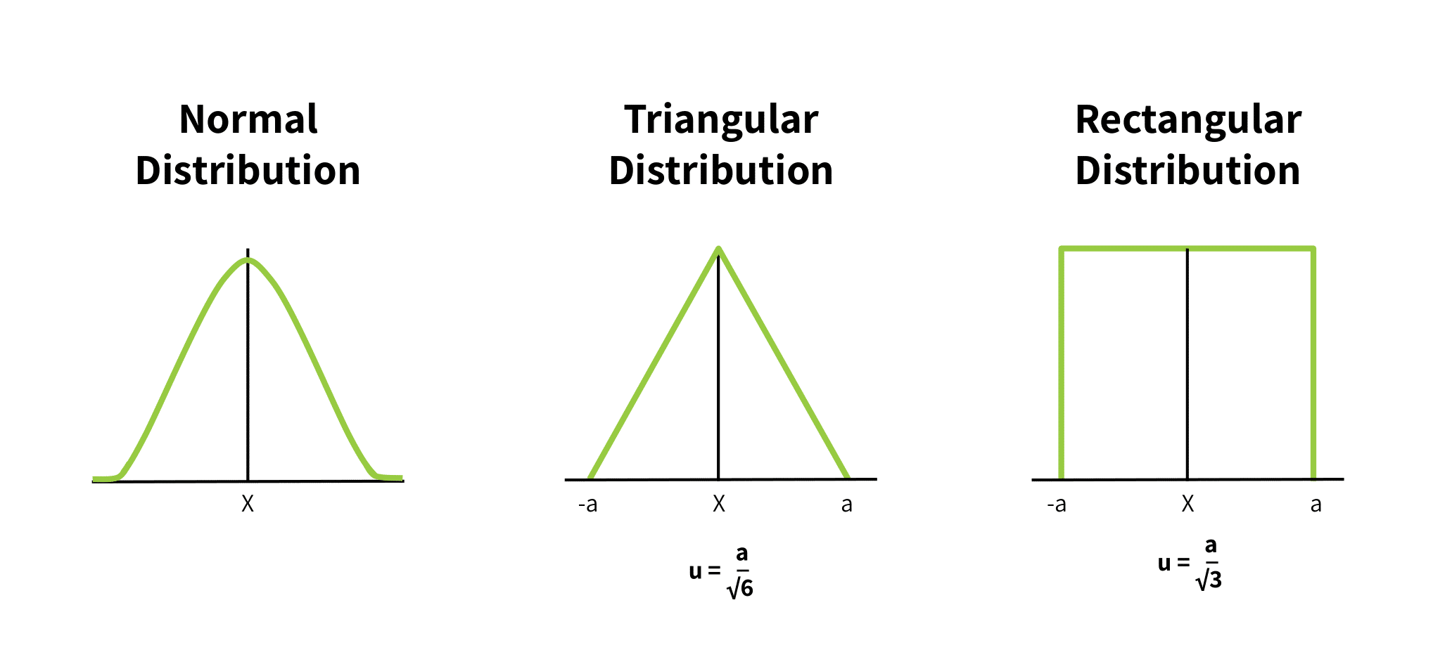
Clearly the normal distribution gives the best picture of uncertainty. However, this involves costly and time consuming experimentation.

A rectangular distribution is appropriate when a given uncertainty does not include a confidence interval. Instead the calculation assumes that all values of the input will fall into a range of values with equal probability. While this is an oversimplification, this assumption gives a valid highest bound of uncertainty, expressed by the equation below the distribution.

A triangular distribution is appropriate when the model of possible true inputs should reflect that values close to the mean are most possible, and the probability of values declines as they get further from the mean. It is an approximation of a normal distribution in the absence of actual measurements. The equation for the standard uncertainty for this assumed distribution appears below the figure.

Step 3: Determining Combined Standard Uncertainty (Propagation of Error)

The most commonly used method for this is the GUM’s law of propagation of uncertainty (LPU). LPU involves the expansion of the mathematical model in a Taylor series and simplifying based on only the first order terms.

The combined standard uncertainty is simply the appropriate combination of standard uncertainties for each input quantity in step 2. The right expression for the combined standard uncertainty depends on whether the input quantities are independently or interdependently correlated. If they are independent, the expression is:

\(u_{c}^{2}(y)=sum_{i=1}^{N}left [ frac{partial f}{partial x_{i}} right ]\)

If they are interdependent, the expression below is added to the right-hand side of the one above:

\(sum {i=1}^{N}sum {j=1}^{N}left [ frac{1}{2} left [ frac{partial^{2} f}{partial x_{i}partial x_{j}} right ]^{2}+frac{partial f}{partial x_{i}}frac{partial ^{3}f}{partial x_{i}partial^{2} {x{j}}}right ]u^{2}(x_{i})u^{2}(x_{j})\)

In the equation above, the partial derivatives are called the sensitivity coefficients. Each of these coefficients is the standard uncertainty of the i-th input quantity. The unsquared value of the product of the partial derivatives with the standard uncertainty is called the uncertainty component.

Step 4: Computing Expanded Uncertainty and Coverage Factors (\(k\))

The expanded uncertainty widens the confidence interval of an expected measurement result. Denoted by (U), it equals the combined standard uncertainty multiplied by an integer known as the coverage factor, (K). Expanded uncertainty ensures the result encompasses a large portion of the distributed values reasonably attributable to the measurand. Mathematically it is:

\(U=Ku_{c}(y)\)

Therefore, the measurement result can be expressed conveniently as (Y = ypm{U}). That is, ((y-U)leq{Y}leq(y+U)). Recall the example of the FSO taken to be as (2.2 mV/V pm0.005 mV/V).

A coverage factor of two gives a confidence interval for the uncertainty of about 95%. Similarly a coverage factor of three gives a confidence interval of uncertainty of about 99.7%. This means the results will fall within the mean result (pm{U}) about 95% or 99.7% of the time respectively.

top

Lab Procedures for Determining Force Measurement Uncertainty

The above are internationally accepted procedures for calculating any measurement uncertainty, per OIML documentation. This section gives an example of how these general procedures are applied in a real life laboratory, in this case the procedures used by NIST to calibrate their own testing equipment and certify manufacturer’s load cells [5].

Example Step 1: Modeling the Measurement Relationship

The polynomial equation that models the force transducer response is:

\(R=A_{0}+ \sum A_{i}F^{i}\)

Where R is the response, F is the applied force and the \(A_{i}\) is the coefficient calculated by applying the least-square fit method to the data set. This equation will become most relevant in step 2 below when we model its uncertainty, which is the third factor (\(u_{r}^2\)) of the combined standard uncertainty above.

Example Step 2: Evaluating the Standard Uncertainty of Each Input

The Uncertainty in Applied Force

The components most significantly contributing to the uncertainty of the applied force (\(u_f\)) are threefold. The uncertainty in the dead weights themselves are one factor. This is because, again, it is impossible to know the true weight of any entity. The remaining factors contributing to applied force uncertainty are the uncertainty in the acceleration due to gravity at the altitude of the test (since force is a function of the mass and gravitational acceleration, or as we learn in high school physics, \(F=ma\)), and the air density at the specific location. These factors may seem minuscule but for very precise systems they are significant and imperative to account for.

The standard uncertainty of the applied force, is then modeled by the equation:

\(u_{f}^{2}=u_{fa}^{2}+u_{fb}^{2}+u_{fc}^{2}\)

where \(u_{fa}\) is the standard uncertainty associated with the mass, \(u_{fb}\) is the acceleration due to gravity, and \(u_{fc}\) is the standard uncertainty due to air density. The value of \(u_{f}^{2}\) is substituted in the combined standard uncertainty equation in step 3 below.

Each of these quantities has been determined by NIST through Type A evaluation for their specific lab location, and can be found in [5].

The Uncertainty of The Voltage Ratio Instrumentation

Recall that force measurement is an indirect measurement. This means the displayed weight is an interpretation of a transducer’s output voltage transducer. (It is not, by contrast, a comparison with a known weight on a balance scale.) This inherently introduces error, since the display or other indicating instrument has its own associated uncertainty.

NIST includes the following standard uncertainty sources in this figure:

In total, the standard uncertainty \(u_{v}\) associated with the instrument is a combination of its sources

\(u_{v}^{2}=u_{va}^{2}+u_{vb}^{2}+u_{vc}^{2}\)

The value of \(u_{v}^{2}\) becomes the second term in the combined standard uncertainty equation in step 3 below. Its value has been derived by NIST using Type A evaluation in their laboratory and can be found in [5].

The Uncertainty Due to the Deviation of the Observed Data from the Fitted Curve

Step 1 above showed that the polynomial equation modeling the force transducer response was:

\(R=A_{0}+ \sum A_{i}F^{i}\)

This equation models what we expect the output of the tested transducer to look like; it is a theoretical model taking into account its electrical components. However, the actual readings from the transducer will deviate from this curve for various applied forces. The differences between the theoretical and measured values for a given input create the standard uncertainty of the response, denoted as \(u_{r}\) and calculated as:

\(u_{r}^{2}=(\sum d_{j}^{: 2})/(n-m)\)

Where \(d_{j}\) are the differences between the measured response \(R_{j}\) and those calculated using the model equation, \(n\) is the number of individual measurements in the calibration data set, and (m) is the order of the polynomial modeling the theoretical output, plus one.

The value of \(u_{r}^{2}\) becomes the third term in the combined standard uncertainty equation in step 3 below. Again, its value has been derived by NIST using Type A evaluation in their laboratory and can be found in [5].

Example Step 3: Determining Combined Standard Uncertainty

Recall from earlier in this document, the combined standard uncertainty is:

\(u_{c}^{: 2}=u_{f}^{: 2}+u_{v}^{: 2}+u_{r}^{: 2}\)

The terms derived in step 2 are placed in this equation, and the combined standard uncertainty, \(u_{c}\), is calculated by taking the square root of each side.

Example Step 4: Computing Expanded Uncertainty and Coverage Factors

Again recall from before, the expanded uncertainty \(U\) is the product of the combined uncertainty \(U_{c}\) and the coverage factor, \(K\). For NIST’s desired confidence interval of 95%, the value of \(K\) is 2, and the expanded uncertainty is therefore:

\(U=Ku_{c}=2u_{c}\).

top

Why Quantifying Force Measurement Uncertainty Matters

We’ve covered how to determine measurement uncertainty. The question is then “why do it?” The following points express the importance of quantifying the uncertainty in force measurements with rigor.

top

Conclusion

Measurement uncertainty is an important concept to understand when selecting and also when calibrating and maintaining load cells. Whereas load cell specification sheets give values of uncertainty, they do not explain their derivation. This article explains globally accepted standard procedures for calculating measurement uncertainty.

As stated before, proper measuring technique and load cell design can lessen the significance of the uncertainty components modeled above. For example proper axial loading, the load cell measurement resolution, the ability to reduce unwanted noise, and the repeatability of the display results all contribute to the deviations in the response vs. the theoretical response curve. Moreover, hysteresis and creep contribute greatly to the uncertainty of the response, \(u_r\), but are controllable with proper maintenance and calibration. (See Calibrating the Force Measuring System and Quality Control: Load Cell Handling, Storage and Preservation Dos and Don’ts.)

In practice, manufacturers design to given, accepted tolerances for a particular class of load cells. (See Load Cell Classes: NIST Requirements and Significant Digit Considerations for Weighing Applications.) Then they specify a load cell measuring range or range of forces that is narrower than the true maximum and minimum capabilities of the load cell. Deviations from expected measurement values are generally more extreme at the limits of the measuring range. Therefore the narrower range ensures the potential errors are well within the bounds of the load cell’s specified tolerances.

top

References