
Choosing a quality multi-axis sensor that meets your specs is just the first step toward creating an accurate measuring device. The four most critical next steps in building a reliable 3-axis (or 6-axis) force measurement system are: (1) mounting the cell within a well-defined coordinate frame, (2) providing one conditioning channel per axis, (3) correcting inter-axis crosstalk with a calibration matrix, and (4) sampling all axes simultaneously so the components stay time-aligned. Done correctly, these steps produce a clean, decoupled \(F_{x}/F_{y}/F_{z}\) (or 6-DOF) signal.
If you are new to multi-axis load cells, we recommend that you start with our introduction, Multi-Axis Load Cells Explained, then return to this guide for its practical steps.
Key Takeaways
- Precise Mechanical Alignment: Align sensor axes cleanly with your system coordinate frame, and torque mounting bolts in a two-stage crisscross pattern to prevent mechanical strain from creating “apparent crosstalk.”
- Matched, Per-Axis Signal Conditioning: Each bridge requires an independent amplifier channel; using matched amplifiers (such as the EMBSGB200 at 5V excitation) ensures consistent filtering, noise rejection, and minimal thermal drift.
- Software-Based Crosstalk Decoupling: Apply the factory 3×3 or 6×6 calibration matrix in software after digitizing to mathematically isolate true orthogonal force vectors from cross-axis channel bleed.
- Time-Synchronous Sampling: Matrix decoupling requires simultaneous sampling across all channels. Asynchronous sampling introduces time-skew (\(\Delta t\)) errors that invalidate matrix math during dynamic loading.
1. Mounting and Alignment: Define Your Axes, Load Point, and Avoid Force Shunts
A multi-axis reading is only meaningful relative to a known coordinate frame. Before connecting anything electrical in the system, follow these steps.
- Fix the cell’s reference frame to the system’s: Choose the critical load point and decide which physical direction is \(+X, +Y, +Z\). Mount the load cell such that its axes and sensing center align with them.
- Mind moment arms: A force applied away from the cell’s measuring center creates moments that introduce error in 3-axis (force-only) load cell measurements. This effect lessens the more the load application point aligns with the sensing center. Alternatively, when moment measurements matter, choose a 6-axis cell instead.
- Avoid unintended force shunts: Over-torqued fasteners or a rigid cable can inject force paths that bypass or bias the load cell.
- Install all mounting hardware meticulously: Because it is part of the load path, not incidental, its proper installation is critical. Be sure to:
- Confirm your load cell’s specific bolt circle, thread size, and torque spec with the manufacturer before assembly.
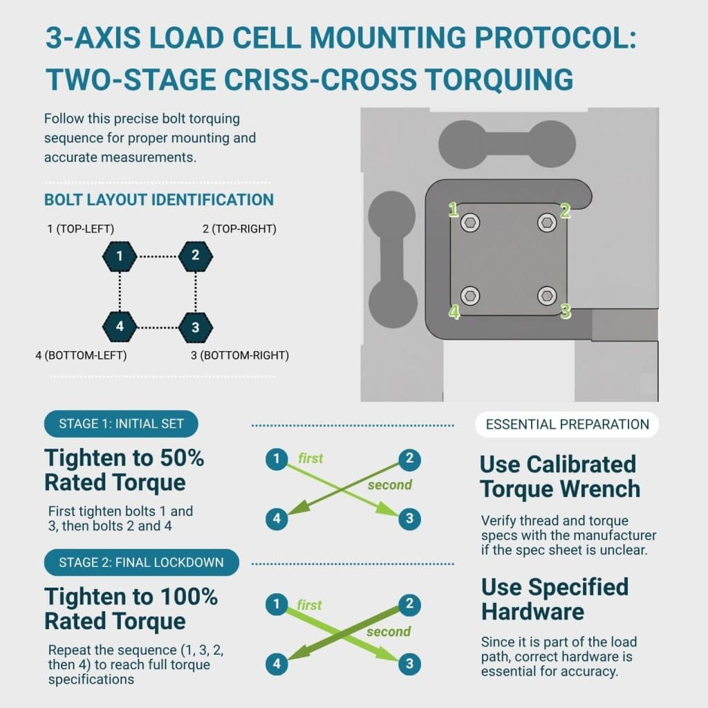
- For multi-bolt cells, torque them in a two-stage crisscross pattern, as shown in the infographic below: tighten the first and third mounting bolts to roughly half the final rated torque, then tighten the remaining two. Follow the same pattern to tighten to full spec.
- Use a calibrated torque wrench, since overtightening distorts the sensing element and permanently shifts the zero point.
It’s imperative to understand that over-torquing matters for multi-axis cells more than for single-axis ones. A mechanical deflection anywhere along the mounting path can introduce apparent crosstalk unrelated to the sensor’s actual cross-axis sensitivity. That is, a poorly torqued bolt can look identical to a calibration problem you don’t actually have.
2. Signal Conditioning: One Amplifier Per Axis
Recall that each measurement axis of the multi-axis load cell is its own strain-gauge Wheatstone bridge. This means each needs its own excitation and its own amplifier/conditioner channel.
Using the recommended pairing of one TSMA 3-axis cell + three identical (model and configuration) EMBSGB200 amplifiers completes the measuring system electronics, with these practical implications:
- The 5V excitation of the EMBSGB200 is a common excitation voltage for modern load cells, and modern instrumentation amplifiers give clean results at that level. Whereas older strain-gauge standards defaulted to 10 V mainly for signal-to-noise reasons, that voltage increases self-heating in the gauges, resulting in increasing thermal drift errors over time.
- Each EMBSGB200 board’s measured excitation and gain values are printed on the bottom. Combined with the cell’s per-axis sensitivity (mV/V), one can derive each channel’s scaling mathematically without trial-and-error:
$$\text{Full-scale output ≈ sensitivity × 5 V × gain} $$
Scale each channel in software by its own known value instead of assuming the three exactly match the theoretical value.
- Choosing the same model and configuration for the three EMBSGB200 units ensures the three have matched filtering, bandwidth, and noise characteristics. This prevents different readings for a fast-changing (dynamic) load on each axis, which skews the load vector’s reconstruction in the final measurement.
3. Crosstalk and the Calibration Matrix
No multi-axis cell has perfectly decoupled axes: a load along one axis still produces a small apparent output on the others. This crosstalk (or cross-axis sensitivity) is characterized at calibration and then removed in software.
Applying the Calibration Matrix
The first-order correction is a matrix multiplication. If the raw bridge outputs are a vector \(v = [v_x, v_y, v_z]\), the true combined force is
\(F = C · v\)
where \(C\) is the calibration matrix supplied with the cell. The matrix size corresponds to the number of output channels: 3×3 for a 3-axis force cell, 6×6 for a full 6-component force/torque cell. The 3-axis equation is as follows:
In other words, for the \(x\) force component,
\(F_x = c_{11}v_x + c_{12}v_y+c_{13}v_z\)
…and so forth.
A note on notation: Each coefficient \(c_{ij}\) describes the effect of axis \(j\) on axis \(i\) — the first subscript is the axis being affected, the second is the axis doing the affecting. The number 1 corresponds to the \(X\) axis, 2 to \(Y\), and 3 to \(Z\). So \(c_{12}\) is “how much Y-axis loading bleeds into the X reading,” while \(c_{21}\) is the reverse — how much X bleeds into Y. These are generally not the same value since crosstalk isn’t necessarily symmetric between two axes.
Thus, the diagonal terms in the calibration matrix are the main per-axis sensitivities. The off-diagonal terms correct the crosstalk. In practice, this matrix multiplication is either handled by your DAQ vendor’s software (many multi-axis sensors ship with a calibration file that’s loaded automatically) or implemented directly in a general-purpose environment like MATLAB or Python. Apply this matrix, and the force vector measurements along each axis are decoupled.
Engineering note: To know what you’re correcting for, it helps to know the scale of the problem. Uncorrected crosstalk in commercial multi-axis cells commonly runs 2–5% of full scale, with under 1% considered excellent performance. Precision cells built for research or calibration work are often specified below 1–2%. Applying the calibration matrix typically reduces that residual crosstalk to a fraction of a percent. It’s also worth knowing that published specs tend to be conservative: in one independent verification, a cell specified at 2% crosstalk at full capacity measured closer to 0.5% in practice. This implies that the number on the datasheet is a guaranteed ceiling rather than a typically-observed field value.
A Caveat for High-Accuracy Work: When the Calibration Matrix Alone is Insufficient
The equation \(F = C·v\) assumes every crosstalk relationship is a straight line, meaning twice the force produces exactly twice the bleed-through on other axes. In real cells, that’s not always true. In fact, the amount of crosstalk can differ depending on whether an axis load is compressive or tensile, since the two directions strain the flexure differently. A single fixed matrix can’t represent that asymmetry since it can only characterize one slope (coefficient) per axis pair. This is why NASA’s three-axis calibration procedure records twelve interaction coefficients per cell rather than the nine in a simple 3×3 matrix—the extra three coefficients capture the difference between positive and negative loading. If this asymmetry matters to your accuracy budget, you’ll need a correction that goes beyond one fixed matrix: either separate corrections for each loading direction (piecewise-linear), or a curve rather than a straight line (polynomial).
Calibration options: Per-axis vs Matrix and Maintenance
For multi-axis load cells, three types of calibration apply: per-axis, matrix, and maintenance calibration.
Per-axis calibration gives you the diagonal sensitivities. This kind of calibration alone is enough when the crosstalk spec is negligible by comparison to your accuracy budget.
Matrix calibration measures the full cross-axis behavior, so it is imperative for accurate off-axis load measurement. However, it is only as good as the calibration rig’s ability to apply a pure single-axis load. Any imprecision in the rig will look identical to crosstalk in the sensor. For this reason, manufacturers typically calibrate each axis independently on a single-axis rig first, which is easier to build with high precision. Doing so gives the baseline reading for that axis and the crosstalk it induces on the others. They then compare this with the combined performance on a separate multi-axis rig to confirm the two agree. The precision in this second step requires purpose-built fixtures, not an improvised rig.
Maintenance calibration keeps the load cell’s calibration matrix accurate over its service life. Setting up a recalibration cycle based on time or usage catches drift before it becomes an unaccounted-for error.
4. Data Acquisition and Sampling
The calibration matrix from the previous section is a snapshot. It is measured once, at a point in time, and remains valid until the sensor’s actual crosstalk behavior drifts away from it due to repeated use (at which point maintenance recalibration becomes necessary). This section covers how you apply a valid matrix to a properly sampled load cell output signal in real time.
That is, both the sampling and the matrix are critical to a meaningful measurement. With a valid matrix but asynchronous samples, the matrix has nothing trustworthy to correct. Meanwhile, use an outdated matrix on perfectly sampled data, and you’re applying accurate math to an outdated sensor model. To avoid these issues, do the following:
- Sample all axes synchronously for dynamic loads. If channels are staggered in time, a moving load “smears” across axes, causing the reconstructed force vector to be inaccurate. A time skew \(\Delta t\) at frequency \(f\) adds roughly \(2\pi f \Delta{t}\) of angular error to the result, and small skews compound quickly at higher frequencies. Simultaneous sample-and-hold matters here in a way it doesn’t for single-axis work, where there’s no second channel to fall out of sync with.
“Smearing” here refers to the result when the matrix multiplies voltages captured at slightly different instances. In this case, the matrix effectively corrects crosstalk between how the load was perceived by one axis at time t and how it affected another at t + Δt. The result characterizes a force that never existed.
For genuinely static or quasi-static loads, sequential sampling with a known skew is acceptable since the skew can be interpolated out after the fact if needed. Synchronization is specifically a dynamic-loading concern.
- Sample each channel fast enough for your force dynamics. Explanations for the underlying sampling rate and anti-aliasing principles appear in our guide, Why Do I Need a Load Cell Amplifier (and Other Signal Conditioners)?. Summarizing here, your DAQ’s sample rate must exceed the Nyquist limit for your fastest expected force transient, or you’ll alias high-frequency events into false low-frequency readings. Choose the same frequency across all channels.
- Filter consistently across axes. Mismatched filtering between channels distorts the reconstructed vector the same way timing skew does, so whatever rate and filter settings you choose, apply them identically to all axes.
- Apply the calibration matrix in software after digitizing, before you interpret \(F_{x}/F_{y}/F_{z}\). The raw channel voltages are meaningless as force values until the matrix is applied. Treat the matrix multiplication as the last step of acquisition, not a separate analysis task performed later. Again, ensure the calibration matrix is up-to-date to prevent an inaccurate result.
Putting it Together: the Bill of Materials
Once you’ve followed these steps to design your 3-axis force measurement system, you can easily build it using the devices in this checklist:
- Our TSMA110 or comparable 3-axis load cell.
- 3× EMBSGB200 amplifiers of the same specifications, for ease of use.
- A synchronous-sampling DAQ with three (or more) analog inputs.
- Software that applies the calibration matrix.
Conclusion
A multi-axis load cell only produces a clean, decoupled force vector when the system around it is built with the same care as the sensor itself. Meticulously following all the steps we covered allows the sensor to produce reliable data throughout its life cycle.
When you are ready to build your system, see our full lineup of TSMA multi-axis load cells and EMBSGB200 amplifiers, or contact us for help specifying a complete measurement stack.