Calibrating the Force Measuring System

All electronic force measuring systems, including industrial weighing systems, consist of a series of components. These components carry the end-to-end signal flow, from the force sensor(s) to the output display or control system. Each of these inevitably introduces error into the final measurement. As the components wear with age, this vulnerability only increases.

Calibration is the process of comparing a system’s actual output signal or weight indication to a known standard and adjusting the system so that it outputs the correct value within an acceptable tolerance. This known standard is simply a very precisely machined test weight, or a machine that applies a settable force, that is directly traceable to an authoritative primary standard. This article explains the end-to-end process of calibrating a force measurement system to ensure absolute accuracy throughout its operational service life.

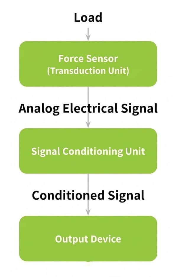
Architecture of an Electronic Force Measuring System

A deployed force measurement system is always the sum of its parts. While routine maintenance calibrations are typically performed on the entire end-to-end apparatus (loop calibration), individual components matter. If a system fails to calibrate within expected tolerances, technicians must isolate and evaluate each component to locate the source of the error.

An electronic force measuring system typically relies on three core stages: Input Transducers, Signal Conditioners, and Output Devices.

How the System Architecture Influences Calibration

Our article, Measurement Uncertainty in Force Measurement, explains the potential errors and theoretical uncertainties inherent in each of these components. Isolating those factors is crucial when a system calibration yields outlier results. However, this guide focuses on calibrating the measuring system as an integrated whole, as loop verification is fundamental to maintaining a deployed field system. By regularly adjusting its output to the expected value within an acceptable tolerance, the system can provide years of accurate, reliable service.

It is important to note that operational calibration tolerances are rarely based solely on the manufacturer’s factory-specified values. Instead, an acceptable tolerance window depends heavily on the specific requirements of the industrial process and the capabilities of the available test equipment.

top

Systematic vs. Random Errors in Deployed Scales

The definition of error is the difference between the measuring system’s output reading and the true value of the measurand. Measurement errors fall into two distinct operational categories: systematic errors and random errors.

Systematic (or Deterministic) Errors

Systematic errors predictably occur during the normal use of measuring devices. The material properties of the internal load cells and system construction largely contribute to these inherent, repeatable errors. Regular calibration and proper measuring system technique can mitigate them considerably.

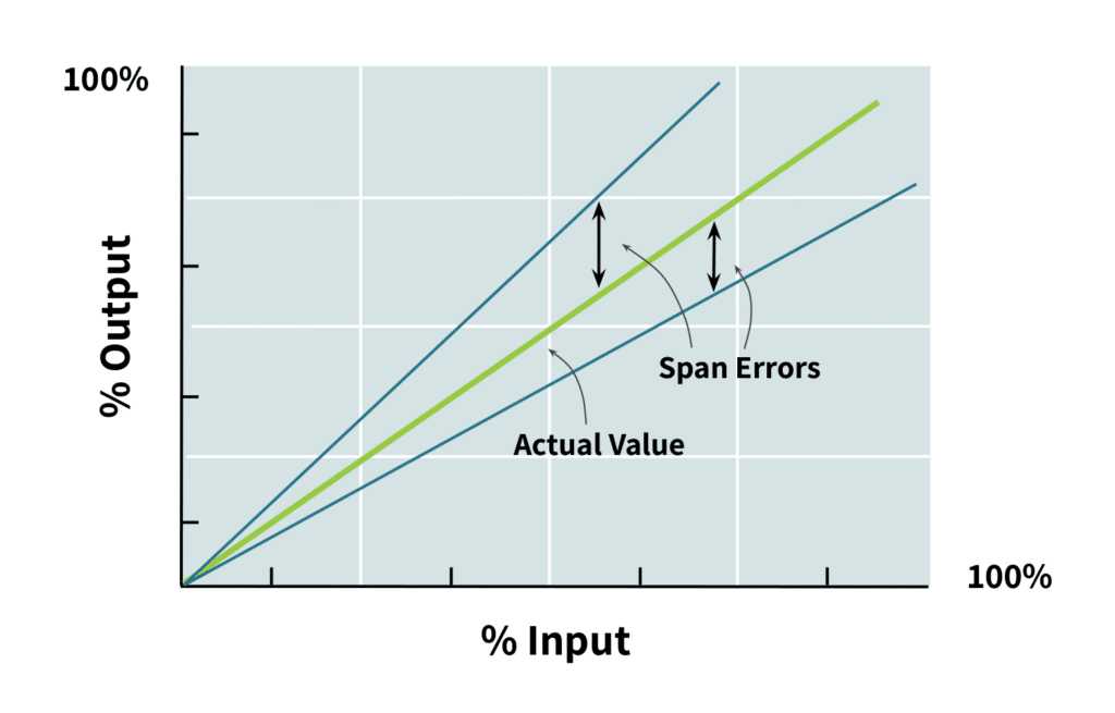
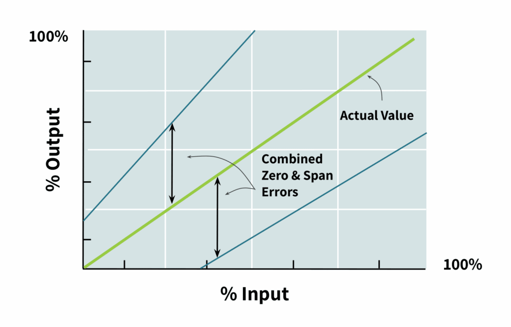
The two main types of systematic errors are zero errors and span errors. These combine to produce a compound systematic error (illustrated in Figure 3) that widens over time.

Zero Errors

Zero errors occur when the system displays a non-zero output despite having no load on the scale. A zero error shifts the entire input-output calibration curve parallel to the true value line, acting as a constant additive error across all weight points. (See Figure 1.)

Span Errors

Span errors alter the slope of the input-output curve. A span error means the measurement discrepancy widens proportionally to the increasing force on the system. (See Figure 2.)

Random (or Stochastic) Errors

Random errors are unpredictable, statistical variations that cause positive and negative fluctuations around a mean measurement value. These variations stem from the precision limitations of the electronics and erratic external environmental shifts, such as transient electrical noise, minor thermal spikes, or ambient building vibrations.

Because random errors are unpredictable, calibration cannot adjust for them. Instead, they are quantified using statistical methods such as calculating standard deviations across repeated test measurements and factored into the total system error.

As the document Measurement Uncertainty in Force Measurement explains, the total system error is then expressed as a mean value plus or minus a stated number of standard deviations within a confidence interval of a given percentage (usually two standard deviations with a 95% or three standard deviations with a 99% confidence interval).

Real-World Sources of Measurement Drift

Whereas calibration can adjust for systematic errors, a proper understanding of their sources can mitigate their presence in the first place. These sources generally fall into two categories: external operational variables and inherent sensor behaviors.

External Operational Variables

• Inconsistent Measurement Methods: If a technician applies a load unevenly, places a weight off-center, or alters the rate of force application between tests, it introduces non-axial loads that distort electrical readings.
• Instrument Calibration Drift: Over extended use, electronic components naturally age, and components like amplifiers and strain gauges slowly drift from their original factory settings.
• Mechanical Lag: Load cells naturally behave like stiff springs; they briefly oscillate under initial loading. Reading a measurement before the sensor has fully reached its steady state results in an artificial error.

Inherent Sensor Behaviors

• Hysteresis: This is a property of the load cell’s elastic element material. The sensor retains a minor mechanical “memory” of applied forces, meaning the voltage output will vary slightly at the same weight point depending on whether the load was reached via increasing force or decreasing force.

top

Environmental & Technical Requirements for Accurate Calibration

The International Society of Automation (ISA) defines calibration as “a test during which known values of a measurand are applied to the transducer and corresponding output readings are documented under specified conditions.” Variations in these four specific conditions outlined by the ISA will introduce stochastic errors that corrupt the calibration test itself.

1. Ambient Conditions

A load cell data sheet lists predicted errors based on tests done under specific ambient conditions. If a measuring system operates in an environment that deviates significantly from the manufacturer’s factory laboratory baselines of the following, it will require specialized compensating electronics or precise field recalibration to ensure accuracy.

• Temperature & Humidity: Thermal fluctuations physically alter the electrical resistance of a load cell’s internal circuitry, skewing the calibration curve. Shifting humidity levels can also compromise insulation resistance in unsealed components.
• Barometric Pressure & Altitude: Because altitude reduces atmospheric pressure, significant elevation differences can reduce the forces on unsealed or uncompensated sensors, altering their baseline output.
• Mechanical & Electrical Noise: Localized machinery vibrations, ambient wind currents, and transient electromagnetic interference (EMI) insert parasitic random noise into millivolt-level sensor output signals.

2. The Force Standard Machine

The force standard machine is the reference apparatus that verifies the testing instruments. To ensure valid mathematical boundaries, this reference equipment must meet strict accuracy and traceability standards:

• The Accuracy Ratio (TUR): To prevent the reference machine from introducing its own excessive uncertainty, its measurement error should be strictly controlled. While a 3:1 ratio (where the machine is three times more accurate than the scale) is sometimes used as a bare minimum field threshold, industry best practice dictates a 4:1 Test Uncertainty Ratio (TUR).
• Metrological Traceability: The reference machine’s accuracy must be verified periodically using a higher-tier standard. This sequence forms an unbroken chain of comparison that must ultimately be traceable to International System of Units (SI) baselines via accredited calibration laboratories and National Metrology Institutes (NMIs) such as NIST in the United States.

3. Technical Personnel Qualifications

Calibration is highly sensitive to operator error. Field personnel must be qualified system technicians who possess a cross-disciplinary understanding of both mechanical and electronic instrumentation. Specifically, technicians must be proficient in:

• Dynamic Control Theory: Understanding how systems respond to live, moving force inputs.
• Analog and Digital Electronics: Managing weak millivolt signals, grounding loops, digital data conversion, and microprocessors.
• Pneumatic, Hydraulic, and Mechanical Systems: Safely executing physical load applications and structural alignments.
• Field Instrumentation: Complete familiarity with field calibration equipment.

4. Operating Procedures for Calibration

Beyond technical knowledge, calibration requires meticulous procedural discipline to satisfy quality management standards like ISO 9000. Technicians must follow a formalized, documented sequence and log every variable in real time. Every calibration record must clearly capture:

• Traceable Device Identifiers: Complete asset information, including the system or load cell serial numbers.
• The Calibration Parameters: The exact weight range tested, specific measurement intervals, and the operational mode used (tension or compression).
• Environmental Metadata: The exact date, time, and ambient environmental conditions present during the test loop.

If an organization lacks the specialized reference equipment or certified personnel required to maintain these strict operating procedures, it should seek professional, manufacturer-backed load cell calibration services.

top

Weighing Standards and Metrological Traceability

In metrology, the term “standards” refers to two separate but related concepts. The first is the documentation that sets forth measuring instrument performance tolerances within a trade jurisdiction (see Load Cell Classes: NIST Requirements, and Load Cell Classes: OIML Requirements).

The other “standards” are undisputed benchmark values of the units of measure (such as precision test weights) against which system accuracy is determined. Every calibration must establish a link through an unbroken chain of comparisons from the test measurand to the highest, universally recognized physical value of that unit. (Standards bodies like OIML warehouse these highest units in highly controlled environments.)

This standards hierarchy has four tiers: the Primary, Secondary, and Working Standards, and the deployed measuring systems themselves. The rule of thumb across the entire chain is the 4:1 rule (the Test Uncertainty Ratio, or TUR). To prevent the higher-tier standard from consuming too much of the lower-tier system’s allowable error, each tier must be at least 4 times more accurate (possessing four times less measurement uncertainty) than the tier directly below it.

1. Primary Standards

Primary standards represent the highest echelon of metrological accuracy. Again, they are maintained exclusively by National Metrology Institutes (NMIs), such as NIST in the United States or the International Bureau of Weights and Measures in France. These institutions use ultra-precise primary deadweight machines to manufacture and maintain national force standards with the absolute lowest possible measurement uncertainty.

2. Secondary Standards

A secondary standard is an instrument or mechanism whose calibration has been established by comparison with the primary force standard. Maintained by accredited calibration laboratories, they serve as the legal calibration vector for industrial equipment.

3. Working Standards

Working standards are the day-to-day tools used by field technicians to calibrate commercial weighing systems. These include certified test weights or dedicated, field-deployable force-applying machines. They must be routinely calibrated against secondary standards to maintain their certified accuracy.

4. Deployed Measuring Systems

The industrial scale, vessel weighing system, or any force sensor operating in a commercial or lab environment sits at the base of the metrological standards hierarchy. It is calibrated directly using working standards.

top

Industrial Calibration Methods & Classifications

Calibration methodologies are classified by what is being adjusted, the scope of the hardware under test, and the environment where the calibration takes place. Technicians must understand these four distinct classifications to execute the correct testing protocol.

1. Zero and Span Calibration (The Adjustment Profile)

This is the fundamental point of calibration: to align the instrument’s input-output measurement curve. Most measuring systems have adjustment knobs or similar for these purposes.

• Zero Calibration: The excitation voltage of a weighing system naturally produces a small residual voltage even when completely unloaded. This baseline signal is caused by inherent electrical imbalances in the sensor’s bridge circuit and the constant physical dead load of the scale structure itself. Zero calibration establishes this residual output as the true baseline, effectively eliminating parallel offset errors.
• Span Calibration: This adjustment sets the 100% full-scale capacity point, tuning the multiplier or “gain” of the electronics to ensure the slope of the measurement curve matches the true value.

2. Individual vs. Loop Calibration (The Equipment Scope)

This classification defines the scope or extent of the testing on the measuring chain.

• Individual Component Calibration: This isolates a single piece of hardware, such as testing a load cell alone on a bench or using a simulator to verify a signal conditioner. This is highly effective for troubleshooting and pinpointing specific component failures.
• Loop Calibration: This tests the entire end-to-end system as a single integrated unit, from the physical force sensor to the digital display. Loop testing is preferable for routine verification because it accounts for combined errors across cables, summing boxes, and instrumentation. Passing loop calibration testing is sufficient for most legal-for-trade applications.

3. Formal Calibration (The Laboratory Benchmark)

Formal calibration refers to the high-precision testing of an accredited calibration laboratory. Examples of devices that must undergo this type of calibration are prototypes of a product line where the manufacturer seeks certification, or devices that will serve as secondary standards.

• This method requires strictly controlled environmental conditions, with completely stable ambient temperature, humidity, and barometric pressure to minimize statistical uncertainty.
• Formal calibration evaluates system components (transducers, displays, etc.) individually using highly precise primary or secondary standards to certify their baseline factory performance.

4. Field Calibration (The Operational Test)

Field calibration is performed on-site after the measuring system has been completely installed in its permanent working environment.

• Field calibration uses portable working standards (like certified test weights) to verify the system under real-world operating conditions. This ensures the system’s outputs are still precise and within maintenance tolerances. (See Load Cell Classes: NIST Requirements for a more detailed description of maintenance tolerances.)
• This step is mandatory because it accounts for structural variables that lab tests cannot see, such as force shunts from attached structures, alterations to load cell cables, and localized machinery vibrations.

top

A Step-by-Step Calibration Procedure for Force Sensors

To satisfy international quality systems like ISO 9000, technicians must execute field calibrations using a highly disciplined, repeatable sequence.

Pre-Test Stabilization (Phase 1)

1. Environmental Verification: Ensure ambient temperature, relative humidity, and barometric pressure are stable and within the sensor’s specified operational boundaries.
2. Mechanical Inspection: Check the load cell mounts for debris, structural binding, or misaligned loading.
3. Warm-Up Cycle: Power on the electronics and allow the system to reach thermal equilibrium according to the manufacturer’s datasheet guidelines.
4. Pre-Loading (Exercising the Sensor): Apply a force near full-scale capacity and release it three distinct times. Exercising the sensor seats the mechanical components and minimizes initial hysteresis and lag during Phase 3.

The Alignment Sequence (Phase 2)

5. Establish the Zero Baseline: Ensure the scale platform has no load, including debris or liquid. If the display shows a residual value, use the instrument’s zero adjustment trim to bring the readout to exactly zero.
6. The Tolerance Guardrail: If the initial zero-load baseline or subsequent span output has drifted by more than one-quarter of your allowable process tolerance limit, stop and perform a formal system adjustment before proceeding with multi-point testing.
7. Apply the Full-Scale Span: Introduce a certified working standard equal to the system’s maximum target capacity. Adjust the instrument’s span or gain setting until the display accurately reflects the known applied load.

Linearity and Repeatability Verification (Phase 3)

8. Stepwise Ascending Test: Apply the working standard weights in uniform increments (typically 5 to 10 equal steps) from zero up to full-scale capacity. To avoid lag errors, allow the observed reading to stabilize before recording it. Record the exact output display at each interval.
9. Stepwise Descending Test: Remove the weights in the exact same descending increments back down to zero, logging the readings at each step. This ascending/descending loop maps the system’s structural linearity and quantifies its operational hysteresis.
10. Repeatability Verification: Repeat the full loading cycle a minimum of three times to verify that the system yields identical, repeatable data points under identical loading conditions.
11. Final Documentation: Log the asset serial numbers, environmental data, “as-found” (pre-adjustment) values, and “as-left” (post-adjustment) values onto the formal calibration certificate.

top

How Often Should a Force Measuring System Be Calibrated?

A force measuring system must be calibrated before its initial field installation. Once a system is actively deployed, operational environments dictate the ongoing maintenance schedule. Calibration every two years is the maximum interval recommended for stable, light-duty applications. Industry best practice typically requires annual recalibration.

Acceleration of this schedule is necessary if the weighing system meets any of the following criteria:

• “Legal for Trade” Requirements: Systems certified for commercial trade must adhere to strict regulatory verification intervals.
• Harsh Environments: Exposure to chronic mechanical shock, corrosive chemicals, washdown moisture, or extreme thermal cycling accelerates component degradation.
• High-Frequency Usage: Systems experiencing continuous or high-cycle loading patterns encounter faster structural and electrical fatigue.
• Data-Driven Drift Trends: Comparing historical calibration certificates from year to year can reveal baseline drift, signaling the need to shorten the window between service intervals.

Conclusion

Routine system calibration is fundamental to reliable industrial data collection. It also forms the core of a preventative maintenance strategy that extends hardware lifespan.

The calibration process generates a detailed calibration curve that charts the precise relationship between a known input force and the system’s electrical output. This performance map quantifies essential operational parameters, including system sensitivity, linearity and hysteresis.

Ultimately, the goal of loop calibration is to ensure that the sensor, cabling, summing box, and instrumentation work in perfect harmony to deliver reliable measurements within acceptable tolerances. If a system fails to calibrate within these required tolerance windows, begin isolating the hardware by following the procedural steps in How to Test for Faults in Load Cells.

Finally, Tacuna Systems offers professional calibration services that can be added to a scale or load cell purchase to ensure optimal operation.

References

• The Calibration Principles.
• The Calibration Handbook of Measuring Instruments by Alessandro Brunelli.
• The Instrumentation Reference Book by Walt Boyes.
• A Guide to the Measurement of Force by Andy Hunt.
• The Standard Practices for Calibration and Verification for Force-Measuring Instruments.
• Force Measurement Services at NIST: Equipment, Procedures, and Uncertainty
• Force Measurement Glossary
• MechTeacher – Generalized Measurement System