Measurement Uncertainty in Force Measurement

This guide outlines standardized methods for evaluating measurement uncertainty in force applications and applies these principles to load cell specification sheets. It synthesizes global practices from leading metrology journals and standard-setting bodies, including the European Association of National Metrology Institutes (EURAMET), the National Institute of Standards and Technology (NIST), ASTM International, and the Joint Committee on Guides in Metrology (JCGM).

While foundational to modern calibration, the formal concept of measurement uncertainty is relatively recent in metrology. Prior to 1977, no international consensus existed for expressing measurement uncertainty [1]. To resolve this ambiguity, the International Committee on Weights and Measures (CIPM) directed the International Bureau of Weights and Measures (BIPM) to collaborate with national laboratories worldwide. Their combined efforts produced the standardized guidelines used today across a vast spectrum of force and mass measurements [1].

The Distinction Between Error and Uncertainty

Often, the terms “error” and “uncertainty” are used interchangeably. However, their distinction is important for quantifying measurement accuracy.

Measurement error is the exact difference between an observed measurement value and the true physical value of the quantity being measured. Crucially, error is a purely theoretical concept that operators can never truly know because it is physically impossible to determine the perfect “true value” of any physical quantity. Improper load cell mounting, mechanical misalignment, or drifting calibration parameters commonly introduce systematic errors into a measurement. While operators can significantly mitigate or correct these errors through rigorous calibration, they can never fully eliminate them.

Measurement uncertainty, on the other hand, does not represent a single value. Instead, it defines a statistically calculated range of values within which the true measurement value is likely to lie, bound by a probabilistic confidence interval. In the weighing world, uncertainty represents a scale manufacturer’s confidence in how close the displayed measurement is to the actual weight on the platform. The next section will illustrate this point further.

Interestingly, the baseline uncertainty models developed by NIST explicitly incorporate physical error variables (sensor creep, hysteresis, and load alignment angle) as a single component of their combined uncertainty. Because clean laboratory procedures can suppress these individual error components, the final combined uncertainty figure in [5] is given as a “best-case” and “worst-case” range. This range directly reflects whether a laboratory operator has actively mitigated those real-world field errors through precise calibration and meticulous execution.

top

How to Interpret Measurement Uncertainty In a Load Cell Data Sheet

As a practical matter, not every application requires the highest possible accuracy, which directly correlates to higher equipment cost. The ultimate engineering goal is to source the most cost-effective tool that still meets the implementation’s accuracy requirements. To achieve this balance, a scale’s or load cell’s datasheet is the authoritative source. Here, we will look at a strain gauge load cell’s uncertainty specification, how it is derived, and what it specifically tells you about the device’s performance.

Statistically Derived Uncertainty and Confidence Intervals

A data sheet specifies a load cell’s output uncertainty as a percentage range of full-scale output (FSO). For example, consider a load cell with an FSO of \(2.2\text{ mV/V} \pm0.25\%\). Mathematically, this \(\pm0.25\%\) tolerance translates to an absolute uncertainty of \(\pm 5.5\ \mu\text{V/V}\), derived by multiplying the percentage by the base output:

\(0.0025 \times (2.2 \times 10^{-3}\text{ V/V}) = 5.5 \times 10^{-6}\text{ V/V}\)

This calculation establishes a highly predictable operational output range spanning from \(2.1945\text{ mV/V}\) to \(2.2055\text{ mV/V}\).

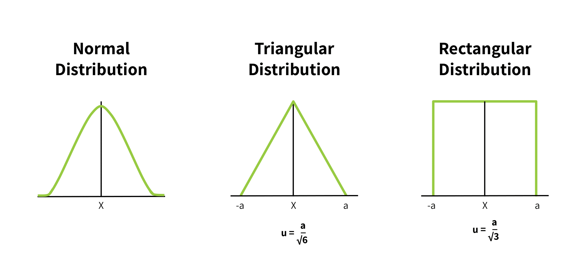
To derive this uncertainty window under ideal conditions, metrologists record a series of repeated measurements using known calibration masses according to standardized international testing frameworks. This experimental dataset maps the exact deviations between the load cell’s actual electrical output and the expected true value. Because these deviations typically follow a Gaussian (normal) distribution around a central mean (see Figure 1a), technicians can apply strict statistical rules to the data.

The uncertainty printed on a commercial datasheet generally represents two or three standard deviations above and below this central mean. When a manufacturer bases their uncertainty on two standard deviations, the load cell will reliably deliver an output within the stated range with a 95% confidence interval. Widening the calculation to three standard deviations expands the boundary lines to guarantee a 99.7% confidence interval.

Returning to our example, the datasheet tells us that the FSO of this specific sensor will fall within the \(2.1945\text{ mV/V}\) to \(2.2055\text{ mV/V}\) window approximately 95% of the time, centered precisely around the baseline \(2.2\text{ mV/V}\) mean. The \(\pm 5.5\ \mu\text{V/V}\) limit represents exactly two standard deviations of the collected sample data. Metrologists refer to the number of standard deviations used to set the confidence interval as the coverage factor (\(k\)), a core parameter detailed later in this guide.

The Economic Reality of Load Cell Accuracy Classes

Conducting this exhaustive, multi-day statistical testing on every single production sensor is financially prohibitive. Instead, manufacturers submit prototype samples to authorized metrology laboratories for type evaluation. This testing certifies that the prototype complies with the performance tolerances of its “accuracy class” set forth by global standards bodies such as OIML and NIST. Note that each regulatory body establishes four to six distinct accuracy classes, ranging from the most restrictive performance limits to wider, utilitarian tolerances, mapping specific target applications to each tier.

Once the prototype is certified, the manufacturer assigns the corresponding accuracy class to that entire model’s production run. This classification explicitly informs buyers which specific tolerance ceilings apply to the performance parameters listed across the device’s datasheet. Consequently, operators can confidently expect real-world output values to remain within these standardized limits provided that ambient temperatures, loading angles, mechanical mounting, and routine maintenance profiles strictly align with manufacturer guidelines.

As NIST notes, tolerance values are carefully balanced so that permissible errors protect against “serious injury to either the buyer or the seller of commodities, yet [are] not so small as to make manufacturing or maintenance costs of equipment disproportionately high [8].”

top

Standard Procedures for Estimating Measurement Uncertainty (The GUM Method)

Evaluating measurement uncertainty follows a rigorous four-step chronological process established by OIML’s Guide to the Expression of Uncertainty in Measurement (GUM) standard [1].

Step 1: Modeling the Measurement Relationship for “Indirect” Measuring

Force measurement is an “indirect” measurement. That is, it differs from a direct measurement, such as checking the width of a pipe with calipers, where the measuring system derives its reading from the pipe’s actual width. Instead, it produces a measurement by converting one form of energy (a physical force) to a different form of energy (an electrical signal), which is filtered, amplified, and processed by an indicator to produce a readable weight value. Each energy transformation introduces a distinct source of measurement uncertainty into the final displayed value.

The GUM Method first mathematically represents the relationship between the measurement output and all of these contributing input quantities. Then, based on these, it models their individual uncertainties to derive the system’s upper bound of combined uncertainty.

The GUM Mathematical Input-Output Equation

Measurement modeling mathematically represents the relationship between the final system output and all contributing input quantities. Metrologists use a strict notation convention to distinguish true values from real-world estimates: uppercase variables represent the actual, ideal values (which are theoretically unknowable), while lowercase variables represent the best available experimental estimates.

The GUM framework expresses the final output value (\(y\)) as a mathematical function (\(f\)) of all individual input components of the measurement (\(x_1, x_2, \dots, x_N\), where the subscript indicates a discrete input out of N total number of inputs):

\(y=f(x_{1},x_{2},…,x_{N})\)

Note that each input component carries a distinct uncertainty associated with its value. Therefore, the combined standard uncertainty associated with the measuring system’s output is likewise a function of these input uncertainties.

Deriving the Combined Standard Uncertainty Model from its Core Components

To compute this cumulative value in practice, the National Institute of Standards and Technology (NIST) models combined standard uncertainty as a function of three core, independent components [5]:

• Applied Force Uncertainty (\(u_f\)): The uncertainty associated with the physical mass standard (i.e., the test weight), localized gravitational acceleration, and air buoyancy (subscript \(f\) for force).
• Instrumentation Uncertainty (\(u_v\)): The uncertainty introduced by the calibration, resolution, and signal processing of the voltage-indicating instrumentation or multimeter (subscript \(v\) for voltage).
• Model Fit Residual Uncertainty (\(u_r\)): The uncertainty derived from how closely the load cell’s calibration data points (or the measured transducer response) fit its best-fit calibration curve, accounting for the residuals (scatter) from factors like hysteresis and non-linearity (subscript \(r\) for residuals).

Because the combined standard uncertainty is a function of the variances of these three independent factors, NIST expresses this relationship through a root-sum-of-squares model:

\(u_c^2 = u_f^2 + u_v^2 + u_r^2\)

The standard combined uncertainty (\(u_c\)) equals the square root of this sum. To transform this baseline standard deviation into a more practical confidence interval, technicians multiply \(u_c\) by a standardized coverage factor (\(k\)). Applying a coverage factor of \(k = 2\) establishes a 95% confidence interval. A factor of \(k = 3\) widens the interval to \(\pm 3u_c\), raising the confidence level to 99.7% that the true value falls within these boundaries.

Modeling the “Ideal” Input Component Value as a Basis for Calculating Uncertainty

Each of these components of uncertainty on the right side of the equation have their own input components that contribute layers of uncertainty. For example, the polynomial equation that models the force transducer’s electrical response curve (used to calculate \(u_r\)) is expressed as:

\(R = A_0 + \sum A_i F^i\)

Where \(R\) represents the transducer response, \(F\) is the applied physical force, and \(A_i\) represents a set of coefficients calculated by applying the least-squares fit method to the calibration dataset. Each test measurement’s deviation from this curve determines the transducer response component (\(u_r\)) of the combined uncertainty (\(u_c\)), as we will demonstrate in the next section.

Step 2: Evaluating the Standard Uncertainty of Each Input Component

In Step 1, we established our high-level system equation:

$$u_c^2 = u_f^2 + u_v^2 + u_r^2$$

Now, in Step 2, we calculate the numerical values of each of these three independent variables (applied force, instrumentation, and curve residuals). We will use the metrologist’s standard notation, \(u(x_i)\) to represent the standard uncertainty, or baseline standard deviation, of whichever one of the three (\(f\), \(v\), or \(r\)) input components (generically represented as \(i\)) is in question.

Per international metrological standards, two distinct methodologies exist to derive these input uncertainties. They are based on the type of data available to the evaluator [7]:

• Type A Evaluation: Uncertainty is calculated through statistical analysis of real-world measurement data. That is, the evaluator has the ability to take repeated measurements of a known weight standard under unvarying environmental conditions.
• Type B Evaluation: The uncertainty is determined via theoretical analysis of historical data, certificates, or physical laws when highly-controlled lab testing is not an option.

Type A Evaluation: Statistical Analysis of Repeated Trials

Type A evaluation translates a series of discrete, real measurements into a standard uncertainty value through a three-step calculation: derive the sample set mean, calculate its standard deviation, and finally, calculate the standard deviation of the mean. To illustrate this, we will use these variables:

• Sample Size, \(n\): The total number of repeated measurements taken during the test (e.g., for 10 measurements of the same calibration deadweight, \(n=10\)).
• Counter, \(k\): This represents the specific trial number currently being calculated (starting at trial \(k=1\) and ticking up sequentially until it reaches \(k=n\)).
• Observed Value, \(x_k\): The raw numerical reading recorded during trial number \(k\) for the specific input component under test. This value is the native output of the tested device, such as a \(\text{mV/V}\) electrical output from a tested load cell, and not the weight reading of an indicator.

The Type A derivation of the final standard uncertainty value (\(u(x_i)\)) follows these steps:

1. Calculate the Sample Mean: This is the basic arithmetic average of all measurement test trials, and represents the best estimate of the real value, \(X\). It therefore becomes the comparison value for calculating how “off” each sample measurement is.

$$\bar{x}_i = \frac{1}{n} \sum_{k=1}^{n} x_k$$

2. Calculate the Experimental Standard Deviation: This measures how far each raw measurement, \(x_i\), strayed from the calculated average \(\bar{x}\).

$$s(x_i) = \sqrt{\frac{1}{n-1} \sum_{k=1}^{n} (x_k – \bar{x}_i)^2}$$

3. Calculate the Standard Uncertainty, or Standard Deviation of the Mean: This is the desired outcome for each component in the uncertainty equation in Step 1. It answers the question: “How accurate is our calculated average?” Notice that as the number of samples (\(n\)) increases, the denominator increases, shrinking the standard uncertainty. This mathematically demonstrates how increased sampling increases confidence in the data.

$$u(x_i) = \frac{s(x_i)}{\sqrt{n}} = \sqrt{\frac{s^2(x_i)}{n}}$$

Type B Evaluation: Theoretical and Historical Data Analysis

This method is essential when repeated testing is physically impractical, economically prohibitive, or logistically constrained. To determine a Type B uncertainty value, metrologists rely on (and clearly state their assumptions for use of) boundary limits from the existing pool of available knowledge:

• Instrument calibration certificates
• Authoritatively published physical constants or metrology journals
• Certified reference materials and manufacturer data sheets
• Documented historical performance data and general engineering knowledge

While Type A evaluation relies on an observed normal distribution (the classic Gaussian bell curve), Type B evaluation models uncertainty using either rectangular or triangular distributions.

Figure 1 shows these distributions. In each, “(a)” is the upper and lower bound of possible values, and \(u(X)\) is the uncertainty around the expected value (the midpoint of the distribution curve).

When a Rectangular Distribution is Appropriate

Metrologists use a rectangular distribution to model uncertainty when an error source specifies a rigid upper and lower limit but fails to provide a confidence interval or a defined distribution shape. This model assumes that every single value within that box has an absolute, equal probability of occurring.

While this is an oversimplification, it provides an intentional conservative upper bound for uncertainty. The standard uncertainty calculation divides the half-interval distance \(a\) by the square root of 3:

$$u(x_i) = \frac{a}{\sqrt{3}}$$

When a Triangular Distribution is Appropriate

A triangular distribution can model the component standard uncertainty when the mathematical representation of possible true inputs indicates:

• that values close to the mean are most likely, and
• the probability of values declines as they get further from the mean.

It is an approximation of a normal distribution where, instead of a bell curve, the probability of an error drops off linearly as the numbers approach the upper and lower measurement limits, \(a\) and \(-a\). The standard uncertainty calculation divides the half-interval distance \(a\) by the square root of 6:

$$u(x_i) = \frac{a}{\sqrt{6}}$$

Case Study Application: How NIST Evaluates Core Input Components

This section gives an example of how Steps 1 and 2 apply in a real-life laboratory. In this case, we show how NIST models the measurement input components (\(f\), \(v\), or \(r\)), and their uncertainties, to calibrate their own testing equipment and certify manufacturers’ load cells [5].

1. Quantifying Applied Force Uncertainty (\(u_f\))

To model the applied force uncertainty (\(u_i\), where \(i = f\)), NIST assigns three distinct force-affecting sub-components:

• Mass Standard Uncertainty (\(u_{fa}\)): The statistical uncertainty associated with the physical mass of the dead weight used for device testing.
• Local Gravitational Uncertainty (\(u_{fb}\)): The uncertainty of the acceleration due to gravity (\(g\)) at the laboratory’s specific geographic coordinates and altitude, since the Newtonian law, \(F=ma\) applies.
• Air Density/Buoyancy Uncertainty (\(u_{fc}\)): The uncertainty introduced by ambient air density variations, which exert a microscopic buoyant lifting force on the dead weights during testing.

These factors may seem minuscule, but for very precise systems, they are significant and imperative to quantify. The resulting force uncertainty equation is:

\(u_{f}^{2}=u_{fa}^{2}+u_{fb}^{2}+u_{fc}^{2}\)

The resulting value of \(u_{f}^{2}\) is substituted for the variable in the combined standard uncertainty equation in Step 3 below.

NIST has recorded values for each of these quantities through rigorous Type A evaluation for each of its specific lab locations. The reference [5] lists these values.

2. Quantifying Instrumentation Voltage Uncertainty (\(u_v\))

Voltage or instrumentation uncertainty exists because, as stated earlier, force measurement is an indirect process. That is, the digits on a display are merely a digital interpretation of a transducer’s analog voltage output. The scale indicator or multimeter introduces its own distinct layer of uncertainty into the measurement.

NIST accounts for this instrument error by combining three distinct sub-components:

• Multimeter Calibration Factor (\(u_{va}\)): The statistical uncertainty tracking the ratio of the multimeter’s displayed voltage relative to a known, certified reference voltage standard.
• Linearity and Resolution Uncertainty (\(u_{vb}\)): The fixed uncertainty dictated by the meter’s internal architecture. This tracks the physical step-size limits of the internal Analog-to-Digital Converter (ADC) along with changes caused by internal component heating and linearity drift over time.
• Primary Reference Calibration (\(u_{vc}\)): The uncertainty derived from calibrating the indicator using a primary transfer standard, such as an ultra-precision electronic load cell simulator.

These factors combine to establish the total instrumentation uncertainty (\(u_v\)) as follows:

$$u_{v}^{2} = u_{va}^{2} + u_{vb}^{2} + u_{vc}^{2}$$

This value becomes the second operational term in the final combined standard uncertainty equation in Step 3.

3. Quantifying Best-Fit Curve Residual Uncertainty (\(u_r\))

As established in Step 1, the mathematical model for the physical force-to-electrical response curve of a force transducer is the polynomial equation:

$$R = A_0 + \sum_{i=1}^{m-1} A_i F^i$$

In this curve model, \(R\) represents the transducer’s electrical response (the raw output value) and \(F\) is the applied physical force. \(A_i\) represents custom coefficients or multipliers derived so that this function’s plot replicates the test sensor’s real-world test data. Note that the \(i\) on the force variable is an exponent, allowing higher-order power terms (like force-squared or force-cubed) to “track” non-linear errors. The variable \(m\) is the coefficient tally, including \(A_0\) (hence the summation counts to \(m-1\)).

During testing, the transducer’s real-world voltage readouts will hover slightly above or below this curve, \(R\), due to factors such as sensor hysteresis and non-linearity. NIST quantifies these differences between the theoretical curve and the actual measured values (\(u_r^2\)) using the following statistical model:

$$u_{r}^{2} = \frac{\sum d_j^2}{n-m}$$

Where:

• \(d_j\): Represents the individual differences (residuals) between the raw measured response (\(R_j\)) and the theoretical value calculated by the polynomial equation.
• \(n\): Represents the total number of individual measurements taken across the calibration run.
• \(m\): Represents the total number of calculated coefficients (\(A_i\), including \(A_0\)) in the electrical response equation. This value is subtracted from the total number of test data points (\(n\)) to determine the residual degrees of freedom (\(n – m\)).

This residual variance (\(u_r^2\)) value becomes the third and final term inside the combined standard uncertainty equation. As with other uncertainties, NIST has quantified baseline values for these that apply to their specific laboratories. The reference [5] lists these values.

top

Step 3: Determining Combined Standard Uncertainty (\(u_c\))

Recall from Step 1, the high-level system variance equation is:

$$u_c^2 = u_f^2 + u_v^2 + u_r^2$$

The combined standard uncertainty (\(u_c\)) of the entire system is simply the Root-Sum-of-Squares (RSS), or the square root of the entire sum to the right of the equals.

$$u_c = \sqrt{u_f^2 + u_v^2 + u_r^2}$$

One simply substitutes the values for the three individual uncertainties derived in Step 2 into this equation and calculates the value.

Step 4: Computing Expanded Uncertainty \(U\) and Coverage Factors (\(k\))

The combined standard uncertainty (\(u_c\)) from Step 3 represents a confidence interval equal to exactly one standard deviation from the mean measurement value. In practical engineering, commercial trade, and industrial safety applications, this window is typically too narrow to be useful. Instead, device specifications give the Expanded Uncertainty (\(U\)), or a wider tolerance of several standard deviations from the mean value.

The Coverage Factor (\(k\))

To scale the uncertainty window, the combined standard uncertainty is multiplied by an integer known as the coverage factor (\(k\)):

$$U = k \cdot u_c(y)$$

By expanding this boundary, the expression of the final measurement shows a realistic tolerance window:

$$Y = y \pm U$$

This mathematically defines the boundaries within which the true value of the measurand (\(Y\)) confidently exists:

$$(y – U) \leq Y \leq (y + U)$$

Connecting Multipliers to Confidence Levels

The choice of the value of the coverage factor (\(k\)) is based on the specific level of confidence required by the testing standard or industry governing body. Assuming a normal distribution of data points across the system, the multipliers expand the reliability net as follows:

• \(k = 2\) (Industrial Baseline): Provides a confidence interval of approximately 95% (specifically 95.45%). This means that if the measurement is repeated under identical conditions, the calculated result will fall within the \(\pm U\) boundary lines roughly 95% of the time.
• \(k = 3\) (High-Certainty Threshold): Widens the confidence interval to 99.73%, mapping out an extreme-precision boundary often required for aerospace or primary laboratory validation.

Recalling the Full-Scale Output (FSO) Example

To connect this back to a real-world example, recall the sensor introduced earlier in this guide, where its Full-Scale Output (FSO) rating was taken to be:

$$2.2 \text{ mV/V} \pm 0.005 \text{ mV/V}$$

In this specification, the \(\pm 0.005 \text{ mV/V}\) represents the definitive expanded uncertainty (\(U\)) of the component.

The goal of conducting a formal calibration run matching NIST’s target standards is to establish a rigorous 95% confidence interval. This ensures the coverage factor of \(k = 2\) is appropriate, and reduces the final system calculation into the simple formula:

$$U = k \cdot u_c = 2u_c$$

top

Why Quantifying Force Measurement Uncertainty Matters

We’ve summarized how metrology experts determine measurement uncertainty that appears in device specifications. The question is then “why this level of rigor?” Quantifying force measurement uncertainty with absolute precision serves several critical engineering, commercial, and regulatory purposes:

top

Conclusion

Understanding measurement uncertainty is important when selecting, calibrating, and maintaining load cells. While load cell specification sheets provide baseline tolerance values, they do not explain their derivation. This guide fills that gap by explaining globally accepted standard procedures for calculating measurement uncertainty.

Ultimately, implementing proper measuring techniques and choosing quality load cell designs can minimize the overall contribution of each uncertainty component modeled here. Proper axial loading, load cell resolution, electrical noise reduction, and repeatable display results all determine how close the transducer response will adhere to the theoretical response curve. Furthermore, hysteresis and creep significantly contribute to the uncertainty of the response, \(u_r\), but are controllable with proper maintenance and routine calibration. (See Calibrating the Force Measuring System and Quality Control: Load Cell Handling, Storage and Preservation Dos and Don’ts.)

In practice, manufacturers design components to fit the accepted tolerances for a particular accuracy class. (See Load Cell Classes: NIST Requirements and Significant Digit Considerations for Weighing Applications.) To protect performance in the field, they intentionally restrict a cell’s specified measuring range to an operational envelope that is narrower than its absolute physical maximum and minimum capabilities. Measurement deviations and non-linear behaviors grow significantly more extreme at the outermost limits of a sensor’s measuring range. Therefore the narrower range ensures the potential errors are well within the bounds of the load cell’s specified tolerances.

top

References