
Every load cell on the market comes with a manufacturer’s data sheet that lists its performance capabilities. These specifications help engineers determine if a load cell meets their application’s requirements. They also serve as a performance benchmark for proper calibration or for identifying faults.
This guide explains how to read a load cell data sheet in three parts: a comprehensive table of performance specs with explanations, a list of physical specifications, and a deeper dive into the most important load cell performance characteristics for those interested in the science behind them.
Key Takeaways
- Master Specification Table: Use the comprehensive matrix below as a fast reference for standard units, brief definitions, and operational notes for 21 core load cell specifications.
- Deep-Dive Performance Metrics: Scroll past the summary table for detailed descriptions of critical specs like FSO, Combined Error, Creep, Thermal Drift, and Overload Limits. This section clarifies subtle differences between similar metrics and reviews how they describe real-world operating conditions and their implications. This understanding of the nuanced behaviors of load cells helps avoid measurement errors and costly structural failures in your system design.
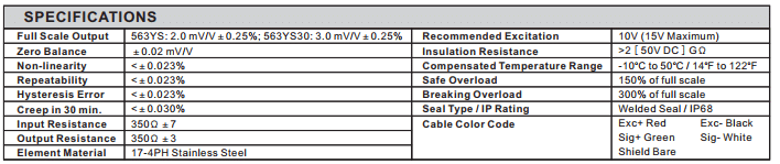
Table of Load Cell Performance Specifications
Performance specs on a load cell data sheet generally cover three areas: output voltage expectations for a given load, the maximum expected error under specific operating conditions, and safe environmental and mechanical operational boundaries.
For some terms below, it may be helpful to refer to Figure 6 in our Force Measurement Glossary. Other definitions in this resource may likewise provide some clarity.
| Specification | Units | Interpretation | Notes |
|---|---|---|---|
| Breaking Overload | % | The ultimate load limit the instrument can withstand before experiencing catastrophic structural failure. | Expressed as a total percentage of rated capacity (e.g., 300% means structural failure occurs under a load 3 times the rated capacity). |
| Combined Error | % | The maximum expected output deviation from a theoretical straight line (voltage output vs. force plot) due to the combined effects of non-linearity and hysteresis. | Expressed as a percentage of full scale output (FSO). |
| Compensated Temp Range | °C to °C °F to °F |
The temperature limits within which the load cell will maintain its zero balance and rated sensitivity specifications. | “Compensated” indicates internal temperature-sensitive resistors have been added to the circuit to offset thermal zero and span drift. |
| Creep in 30 minutes | ± % | The change in output signal occurring over time while under a constant, continuous load (typically rated capacity) with all environmental factors held constant. | Expressed as a percentage of full scale output (FSO). |
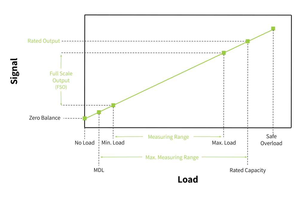
| Full Scale Output (FSO) | mV/V | The output voltage the load cell produces at rated capacity, minus the output voltage at minimum load, per excitation volt at the input terminals. | Multiply the FSO by the excitation voltage to calculate the total expected voltage swing from a zero-load state to full capacity. |
| Hysteresis Error | ± % | The maximum difference between ascending-load and descending-load output voltage readings at the exact same load point across the measurement range. | Expressed as a percentage of full scale output (FSO). |
| Input Resistance | Ω | The electrical resistance of the load cell’s internal excitation circuit. | Measured across the input terminals under no load conditions and an open circuit at the output. |
| Insulation Resistance | GΩ | The electrical resistance measured between the internal circuit bridge and the physical structure (body) of the load cell. | High insulation resistance (typically 5 GΩ or greater) prevents stray voltage leakage and signal degradation. |
| IP Rating | “IP” + 2 digits | A standardized classification indicating the level of environmental protection a load cell’s coating or structure provides against solids and liquids. | Ratings use two digits (e.g., IP68); the first digit measures solid particle protection and the second measures liquid ingress protection. See this useful graphic. |
| Non-linearity | ± % | The maximum output voltage deviation from a theoretical linear input-output plot at any load between zero and rated capacity. The comparative theoretical linear input-output function is the line from zero balance output at no load to output at max load. | Expressed as a percentage of full scale output (FSO). |
| Output Resistance | Ω | The electrical resistance of the internal output signal circuit. | Measured across the output terminals under no-load conditions with an open circuit at the input. |
| Rated Capacity | Mass or force units | Maximum load the device can bear and still perform within its rated tolerance limits. | Expressed in standard engineering units such as lbs, kg, tons, or Newtons, depending on the specific load cell’s scale. |
| Recommended Excitation | V | The optimal input voltage required to power the internal strain gauge bridge circuit. | Usually listed as a baseline value along with a maximum allowable voltage limit (e.g., 10V Recommended, 15V Max). Load cells are passive devices; therefore, all require excitation voltage. |
| Repeatability | ± % | The maximum difference between output readings when the exact same load is applied repeatedly under identical environmental and loading conditions. | Expressed as a percentage of full scale output (FSO). |
| Safe Overload | % | The maximum total load an instrument can withstand without experiencing a permanent mechanical shift in zero balance or performance beyond its specifications. | Expressed as a total percentage of rated capacity (e.g., 150% means the cell can take on a load 1.5 times its rated capacity without causing permanent deformation). |
| Sensitivity | mV/V | The ratio of the change in output signal voltage to the change in the applied mechanical load. | For an unamplified load cell, sensitivity is numerically identical to its Full Scale Output (FSO). It is a measure of signal strength. |
| Service Temperature Range | °C to °C °F to °F |
The environmental temperature limits within which the load cell can safely operate without sustaining permanent damage. | This range is wider than the Compensated range; performance errors will likely exceed standard datasheet tolerances when operating in this zone. |
| Storage Temperature Range | °C to °C °F to °F |
Ambient temperature limits while the load cell is in storage. | Storage within these limits will prevent permanent calibration shifts affecting performance when the load cell is redeployed. |
| Temperature Effect on Sensitivity | ±% of load per °C | The change in rated output (span) sensitivity caused by fluctuations in ambient temperature. | This error only impacts the reading when the load cell is under load. It represents thermal span drift. |
| Temperature Effect on Zero Balance | ± % FSO / °C | The shift in the baseline zero-load output signal caused by fluctuations in ambient temperature. | This error causes the scale’s tare or zero point to drift up or down even when the scale is completely empty. |
| Zero Balance or Zero Offset | mV/V | The electrical output signal produced by the load cell under a true no-load condition, per volt of excitation. | Tells you how far off from a perfect 0.00 mV/V the unfiltered sensor sits before first in-service calibration. |
Other Load Cell Data Sheet Specifications
Beyond the sensor performance specifications, data sheets also include some of the device’s physical characteristics.
- Dimensions: The spec sheet has a CAD drawing with dimensions (height, width, length, mounting hole circumference, etc.) labeled as variables. A table follows that lists the value of each dimension for each rated capacity option.
- Material: The load cell spring element material appears, since different materials perform differently over time depending on the environmental conditions.
- Cable Color Code: Load cell wire coloring is not standardized. Therefore, data sheets always specify which color wire is the positive and negative excitation, positive or negative signal output, and in 6-wire configurations, the positive and negative sense wires. These are labeled as follows:
| Wire Name | Datasheet Code | Used In |
|---|---|---|
| Positive Excitation | Exc+ | 4-wire & 6-wire |
| Negative Excitation | Exc- | 4-wire & 6-wire |
| Positive Signal | Sig+ | 4-wire & 6-wire |
| Negative Signal | Sig- | 4-wire & 6-wire |
| Positive Sense | Sense+ | 6-wire only |
| Negative Sense | Sense- | 6-wire only |
Note: Where long cable runs are necessary, use a 6-wire load cell with sense wires. The dedicated sense wires actively monitor the excitation voltage at the load cell, canceling out measurement errors caused by voltage drops in the cabling. You can read more about this in our article, External Wiring in Strain Gauge Load Cells.
Interpreting Key Load Cell Data Sheet Performance Metrics: The Subtleties
While the specification table provides a quick reference, a deeper understanding of how certain key performance metrics interact in real-world applications is useful. The following sections break down the most critical performance indicators on a manufacturer’s datasheet, in logical groupings.
1) Design Implications of Full Scale Output (FSO) and Sensitivity
On a manufacturer’s datasheet, Full Scale Output (FSO) and Sensitivity are used interchangeably and have the same numerical value (usually \(2.0\text{ mV/V}\) or \(3.0\text{ mV/V}\)). They describe the ratiometric relationship between the input excitation voltage and the final output signal at maximum capacity. This value then allows you to calculate the output voltage in mV per unit of force (lbs, kg, N).
Calculating the Output Voltage Swing
To design the downstream electronics, engineers must know the total signal span available across the sensor’s entire weight capacity.
Multiplying FSO by your excitation voltage gives you the exact signal span from an unloaded state to its maximum rated capacity. The calculation is:
$$\text{Voltage Swing (mV)} = \text{FSO (mV/V)} \times \text{Excitation Voltage (V)}$$
Therefore, a load cell with a \(2.0\text{ mV/V}\) sensitivity powered by a \(10\text{V}\) excitation voltage will yield a net output of \(20\text{ mV}\) at full capacity.
Converting to Per-Engineering-Unit Sensitivity (mV/unit of force)
This full-scale voltage swing informs the downstream electronics of exactly how many millivolts the bridge outputs per unit of force (or per-engineering-unit sensitivity). In this example, we will use pounds:
$$\text{Per-engineering unit sensitivity (mV/lb)} = \frac{\text{Voltage Swing at Full Scale (mV)}}{\text{Rated Capacity (lbs)}}$$
Let’s assume a load cell with 1000lb rated capacity has the full-scale voltage of 20mV:
$$\text{Per-engineering unit sensitivity (mV/lb)} = \frac{\text{20 mV}}{\text{1000 lbs}} = \text{0.02 mV/lb}$$
An instrumentation programmer inputs this final \(0.02\text{ mV/lb}\) scaling factor into the indicator or data collection software, so the system can accurately translate real-time voltage changes back into weight metrics.
Back to Summary Table2) Quantifying the Cumulative Effects of All Error Sources
The previous section describes a perfect, linear relationship between a load cell’s input and output. In reality, the materials used in sensor construction exhibit minor deviations in their elastic behavior that affect this ideal line. Some of these errors are quantifiable in an instant (static errors), and others appear as a drifting measurement over time. Other errors are more random in nature.
For a deeper explanation, see Measurement Uncertainty in Force Measurement and Calibrating the Force Measuring System.
Static Measurement Errors
Again, these errors are inherent to the sensor materials and occur predictably. Datasheets quantify these deviations using these interrelated metrics:
- Non-linearity: The maximum deviation of the output signal from a theoretical straight line drawn between zero load and rated capacity during an increasing load test.
- Hysteresis Error: The maximum difference between ascending-load and descending-load voltage output readings at the exact same weight point.
- Combined Error: A comprehensive metric where the manufacturer bounds the worst-case effects of both non-linearity and hysteresis into a single accuracy window.
Using Combined Error simplifies your system math. If a load cell data sheet gives a combined error of \(\pm0.03\%\) of FSO, you can quickly calculate the maximum expected measurement deviation across the entire operating range due to spring element behavior.
Load Cell Creep and Time-Dependent Drift
Creep is the change in the output signal that occurs over time while a load cell remains under a constant, continuous load with all environmental variables held completely steady. Per NIST Handbook 44 guidelines, datasheets list this as a maximum percentage of FSO over a 30-minute interval.
Creep occurs due to the microscopic, time-dependent strain properties of both the metal spring element and the adhesives bonding the strain gauges to it. Understanding creep is vital for static weighing installations such as tank, silo, or hopper batching systems, where materials sit on the scale for extended periods before processing. If creep limits are too high, the signal will slowly drift, recording an artificial change in weight.
Repeatability Errors
Repeatability measures how consistently the sensor returns to the same value during back-to-back trials under identical conditions. Manufacturers represent repeatability errors separately since they represent statistical randomness and electrical or mechanical noise, rather than a predictable input-output curve. The data sheet’s repeatability figure shows the absolute worst-case spread between the highest and lowest readings in factory testing. It defines the maximum boundary of that randomness.
External application variables such as mounting friction, slight structural misalignments, or ambient vibrations heavily influence repeatability. If a datasheet guarantees a repeatability of \(\pm0.02\%\) FS, but your installed scale shows a random variation of \(\pm0.10\%\) FS during testing, the problem is most likely not the sensor. Instead, the culprit is external system noise, such as mechanical binding in the weigh module, structural deflection, or electrical interference on the cable run. Troubleshooting can verify this.
Calculating the Combined Error Budget
While datasheets list these error components individually, system performance depends on their concurrent interaction. Engineers calculate this error budget using two distinct methods.
Note: This budget excludes temperature coefficients because thermal drift stems from external environmental shifts rather than the sensor’s baseline mechanical properties.
Method 1: The Worst-Case Algebraic Sum
This conservative approach assumes that every mechanical error simultaneously pulls the signal in the same negative or positive direction. Engineers use this formula when designing high-risk or safety-critical systems where they cannot afford to underestimate potential error propagation:
$$\text{Total Static Error} = \text{Non-Linearity} + \text{Hysteresis} + \text{Repeatability} + \text{Creep}$$
Method 2: The Root Sum Square (RSS) Estimate
In real-world field applications, it is improbable that all independent, random mechanical errors peak at the same moment in the same direction. The Root Sum Square (RSS) method provides a more statistically realistic error budget estimate:
$$e_{RSS} = \sqrt{e_{NL}^2 + e_{hys}^2 + e_{rep}^2 + e_{creep}^2}$$
Back to Summary TablePro-Tip: If your datasheet provides a pre-calculated “Combined Error” value from the manufacturer, you can substitute the square of that single percentage for the sum of the squares of non-linearity (\(e_{NL}\)) and hysteresis (\(e_{hys}\)) terms to streamline your total RSS calculation. The square of their worst-case algebraic sum is greater than the sum of their squares, so using this value in a Root Sum Square (RSS) formula creates a “conservative estimate.”
4) Temperature Effects: Thermal Zero Shift vs. Thermal Span Drift
Temperature fluctuations physically alter the electrical resistance of a load cell’s internal circuitry and the elasticity of its metal body. Datasheets give these thermal impacts as two separate metrics because they affect the measurement curve differently:
- Temperature Effect on Zero Balance: This shifts the baseline starting point of the entire measurement curve up or down. It acts as a constant, additive error that is present even when the scale is unloaded. Because it is static at any given temperature, this effect can be eliminated in the field by pressing a scale’s Tare button before beginning a measurement cycle.
- Temperature Effect on Sensitivity (Thermal Span Drift): This alters the slope or multiplier of the measurement curve. It changes how much the signal reacts per unit of force. This error is undetectable when the scale is unloaded, but scales up linearly as more weight is added. It cannot be corrected by taring the scale.
These errors can very quickly exceed the error budget we calculated in the last section. For example, assume a 20° temperature change and \(0.002\%/^\circ\text{C}\) for each temperature effect figure.
$$e_{\text{temp}} = (\text{TCS} + \text{TCZ}) \times \Delta T$$
Substituting,
$$e_{\text{temp}} = (0.002\%/^\circ\text{C} + 0.002\%/^\circ\text{C}) \times 20^\circ\text{C} = 0.08\%\text{ FS}$$
This is greater than the typical sum of all the other error figures.
Manufacturers add temperature-sensitive resistors directly into the internal bridge circuit to minimize these variations across the listed Compensated Temperature Range. Operating your scale within this temperature range will ensure the greatest measurement accuracy.
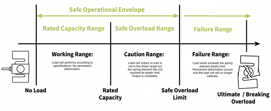
Back to Summary Table5) Structural Overload Limits: Safe vs. Breaking Overload
Overload specifications establish the definitive physical boundaries for protecting your equipment from unexpected forces, such as wind loads, mechanical binding, or shock loading.
- Safe Overload: The maximum total load an instrument can withstand relative to its capacity before experiencing permanent structural distortion. For instance, a safe overload spec of \(150\%\) means a \(1,000\text{ lb}\) load cell can briefly experience a total absolute load of \(1,500\text{ lbs}\) without permanent damage. Exceeding this limit causes the load cell body, or elastic element, to cross into the material’s inelastic range on its stress/strain curve. This will cause a permanent mechanical shift in the zero balance, requiring recalibration or component replacement.
- Breaking Overload: The ultimate structural limit before catastrophic physical failure occurs, relative to the rated capacity. A breaking overload spec of \(300\%\) means the sensor body of a \(1000\text{ lbs}\) rated capacity will physically shear, buckle, or fracture at \(3,000\text{ lbs}\) of total absolute force. Clearly, this poses an immediate structural safety risk to the entire weighing assembly.
This figure illustrates the difference.
Conclusion: How Load Cell Specifications Apply to Your Project
It may seem somewhat intuitive, but applying the numbers in the spec sheet simply amounts to making sure the performance they describe matches your project requirements. Can the load cell operate in the ambient temperatures where it would function? Can it handle the humidity and particulate matter in the weigh system’s environment (see “IP rating” in the table)? Is the sensitivity appropriate for your signal conditioner and display? (See “How does a load cell’s sensitivity relate to the display or interface I choose?” in our FAQs.) These and similar questions make knowing how to read a load cell data sheet important to any weigh system design.
For more information on these data sheet specifications, see What is the Lowest Weight a Load Cell Can Measure?. For more guidance on selecting weigh system components, see our popular article, Choosing the Right Load Cell for Your Job. Or use our contact form to request project-specific consultation.
References
- Scale Manufacturers Association (SMA), Load Cell Application and Test Guideline
- Rice Lake Weighing Systems, Load Cell and Weigh Module Handbook
- Rice Lake Weighing Systems, Load Cell Handbook
- International Organization of Legal Metrology (OIML), OIML R 60-1